Prediction
Intuition
Raster image can have very large spatial resolution. It is impossible to input whole raster image as an input to model because of constrain about memory and time, instead approch like split raster into sub-patch and make prediction independent together then mosiac back to original size is often use. But the problem is at the boundary of each patch will lost information of adjacent patch and cause error in convolutional operation.
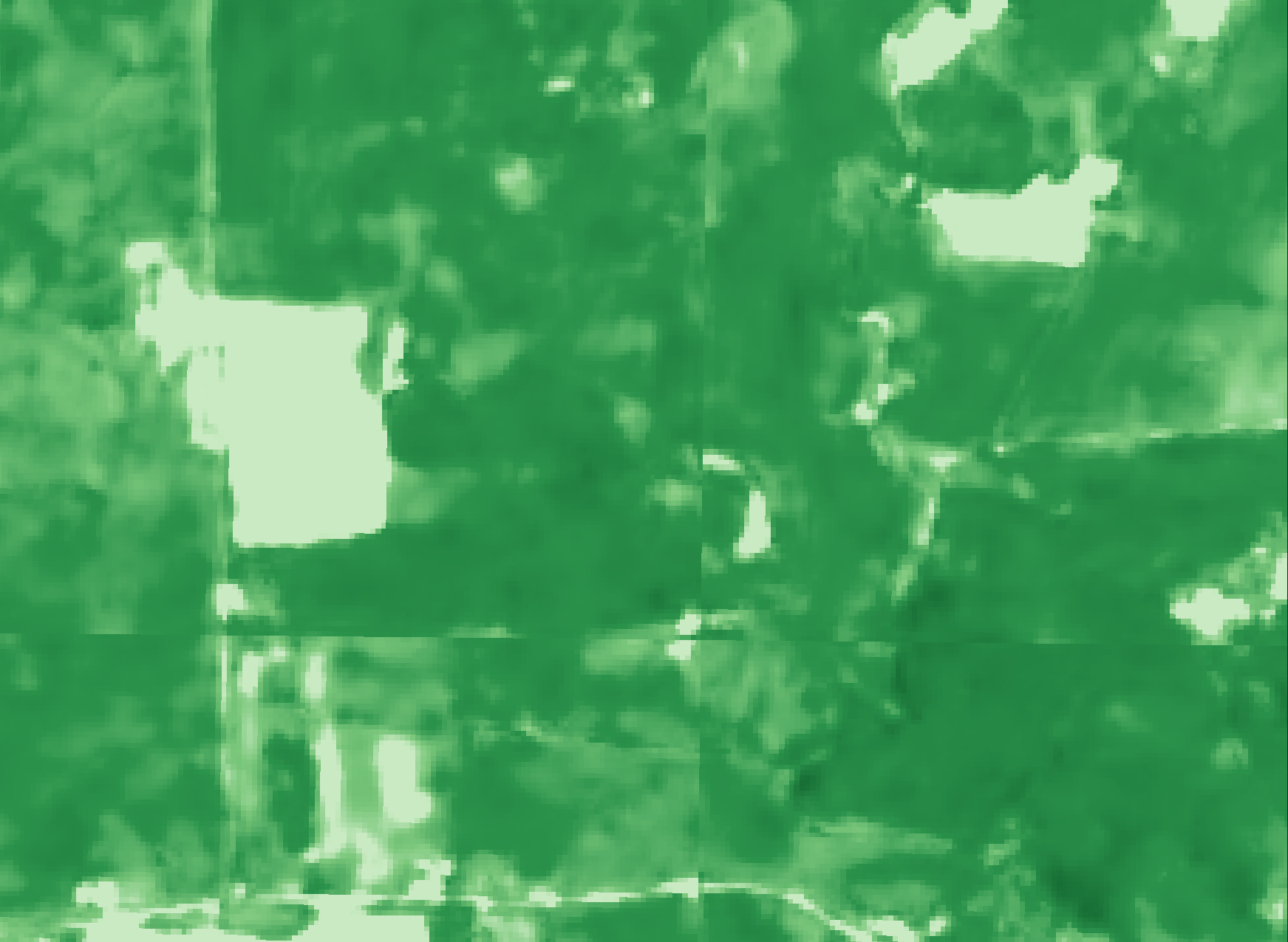
Figure : Example of boundary error when prediction raster image by sub-patch
Another apporch that solve this problem is use averaging sliding window technique. We implement by make a prediction by some fixed sized window. Then step the window by the number of stride , some pixel will be overlap from previous prediction. We process by accumulate the prediction and using using extra accumulator array to count the number of redundant prediction. After prediction is finised. We then divide the accumulate prediction result with accumulator number of each pixel to get average prediction. Results mitigate the error at the boundary.
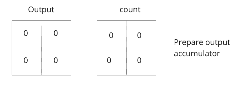
Figure 1 : Initial state of output and accumulator, no prediction takes place yet.
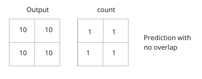
Figure 2 : First window prediction, accumulator count the number to total prediction
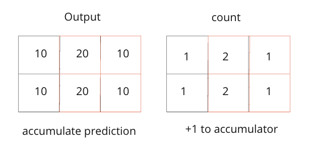
Figure 3 : Sliding window move by stride number, some pixel make prediction agian, accumulate the prediction and count total number of prediction.

Figure 5 : By the end of operation , divide total accumulate prediction with the number of prediction to get average result.
Prediction
Prediction on one model
predict_model.py implement averaging sliding window technique as state before.
Right now we should have total of n candidate ensemble. predict_model.py use make prediction for each model by using raster file as input directly and produce raster output.
Input :
Sentinel 2 + 1 stack rasterimage
14 channel .tif or tiff same band arrangement as training image
Output :
1 channel output prediction, raster image (.tif)
1 channel variance of output prediction, raster image (.tif)
Usage
python3 predict_model.py [--model_path MODEL_DIRECTORY] [--input INPUT_FILE_PATH] [--output OUTPUT_FILE_PATH]Note : MODEL_DIRECTORY , Specify the path in which the candidate ensemble model best_weights.pt is stored
You can define window size and stride in optional argument.
More stride will get more accurately result but increase time complexity.
More window size speed up inference time if you have enough computational resource.
optinal arguments:
  --channels num_ch         Number of input_channels , default=14
  --bilinear BL             Use bilinear upsampling,  default=True
  --window_size WINDOW      Define size of window , default = 2096

  --stride STIRDE           Step size for window sliding  , default = 2000
Merge ensemsble prediction
To produce final output of ensemble prediction. We implement methodology state in uncertianty section.
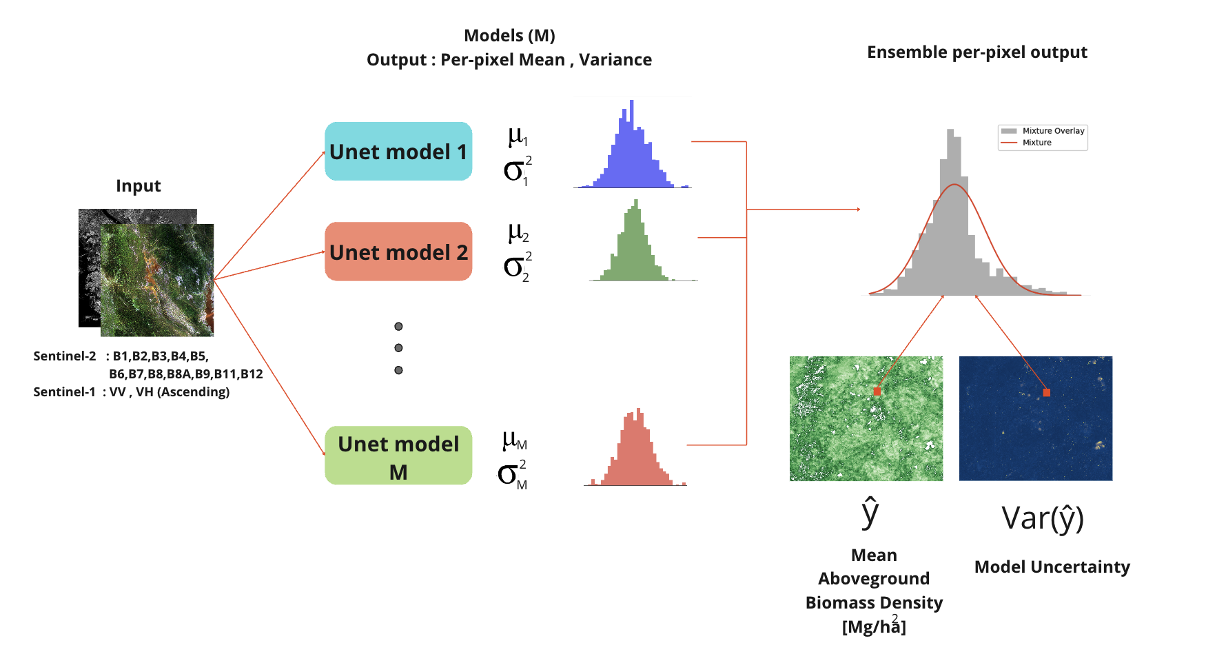
Figure : Inference flow of the ensemble model.
- Prepare all output prediction and variance of all candidate ensemble
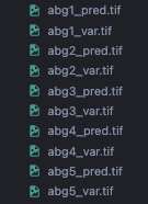
Figure : collection of output prediction and variance of all candidate ensemble
- Stack output prediction and varaince
Since output and total variance equation require pixel wise summation and average operation. If computational resource is limited, we can calculate by subset of array.
For simplicity of demonstration, AGB output and varince has 1 dimensional so we stack whole image together
We can use numpy and rasterio(for reading raster)
import numpy as np
import os
import glob
import rasterio as rio

rootdir = path/to/emsemble/collection

predict_pattern = "abg**_pred**"
variance_pattern  = "abg**_var**"

predict_file  = glob.glob(os.path.join(rootdir, predict_pattern))
variance_file  = glob.glob(os.path.join(rootdir, variance_pattern))

predicts_img = np.array([rio.open(file).read() for file in predict_file])
variances_img = np.array([rio.open(file).read() for file in variance_file])- Pixel-wise average output predictions
- Avarage of output can be implement be numpy.mean
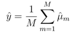
Output Equation : output prediction of the model , calculate by averaging each pixel for all M candidate
# final predictions (average over model ensemble)
pred_ensemble = np.mean(predicts_img, axis=0)- Calculate Pixel-wise epistemic uncertainty (model uncertainty) of ensemble model
- Can be done by calculate pixel-wise varince of all output predictions
epistemic_var = np.var(predicts_img, axis=0)- Calculate Pixel-wise aleatoric uncertainty (data uncertainty) of ensemble model
- Can be done by calculate pixel-wise avarage on all variances of ensemble
aleatoric_var = np.mean(variances_img, axis=0)- Combine epistemic and aleatoric uncertainty
- Pixel-wise summation epistemic and aleatoric uncertainty according to total variance formula
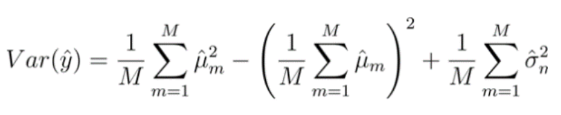
Total Variance Equation : Epistemic (terms 1 and 2) + Aleatoric Uncertainty (term 3) Uncertainty
predictive_var = epistemic_var + aleatoric_var- Write result numpy array to raster image.
- Using rasterio to get raster metadata from any output prediction(same geodata)
img_tmp = rio.open('path/to/emsemble/collection/abg1_pred.tif')
out_profile = img_tmp.profile.copy()
out_profile.update(count=1)

dst_prediction = rio.open('path/to/emsemble/output/ensemble_pred_AGB.tif', 'w', **out_profile)
dst_var = rio.open('path/to/emsemble/output/ensemble_variance_AGB.tif', 'w', **out_profile)

dst_prediction.write(pred_ensemble)
dst_var.write(predictive_var)

dst_prediction.close()
dst_var.close()