GEDI

Overview

The Global Ecosystem Dynamics Investigation (GEDI) spaceborne lidar, which produces high resolution laser ranging observations of the 3D structure of the Earth. GEDI’s measurements of surface elevation and vegetation canopies allow for precise estimates of canopy height and vertical structure, facilitating research applications and policy implications that have long been anticipated by the global terrestrial ecology and carbon cycle science communities.

GEDI science data products include footprint and gridded data sets that describe the 3D features of the Earth. These data products are assigned different levels, which indicate the amount of processing that the data has undergone after collection. All products are publicly available, with the lower level products (L1 & L2) from NASA’s Land Processes Distributed Active Archive Center (LPDAAC) and the higher level (L3 & L4) from the ORNL DAAC. Data are initially transferred to the GEDI Mission Operations Center (MOC) at the Goddard Space Flight Center that deploys acquisition planning on a weekly basis, and then processed through the Science Operations Center (SOC) to distribute science data products to the above DAACs.

The physical theories, mathematical procedures and model assumptions that are used in the creation of these data products are described in the Algorithm Theoretical Basis Documents (ATBDs). These can be found here.

GEDI Product

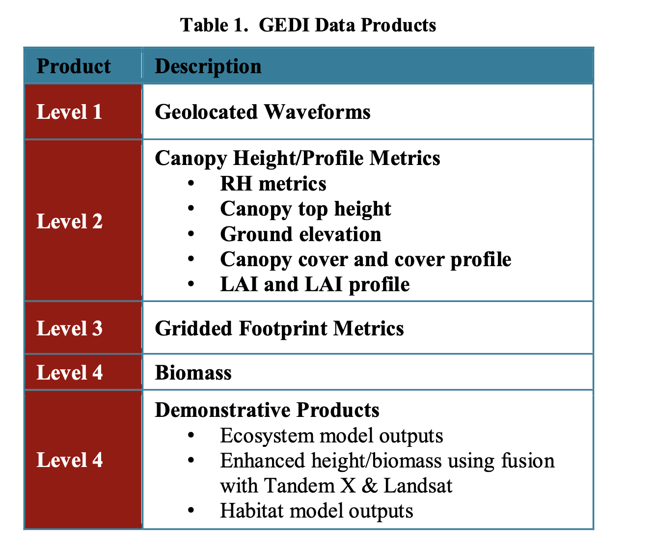
LEVEL 1 - GEOLOCATED WAVEFORMS

The raw GEDI waveforms as collected by the GEDI system are geolocated by our science team.

• The GEDI Level 1 data products are developed in two separate products, a Level 1A (L1A) and a Level 1B (L1B) product.

1. The GEDI L1A data product contains fundamental instrument engineering and housekeeping data as well as the raw waveform and geolocation information used to compute higher level data products.
2. The GEDI L1B geolocated waveform data product, while similar to the L1A data product, contains specific data to support the computation of the higher level 2A and 2B data products. These L1B data include the corrected receive waveform, as well as the receive waveform geolocation information. The L1B data products provide end users with context for the higher L2 products as well as the ability for end users to apply their own waveform interpretation algorithms.

LEVEL 2 - FOOTPRINT LEVEL CANOPY HEIGHT AND PROFILE METRICS

The L2 products contain information derived from the geolocated GEDI return waveforms (Level 1 product) .The waveforms are processed to provide canopy height and profile metrics. These are values calculated directly from the waveform return for each footprint such as terrain elevation, canopy height, RH metrics and Leaf Area Index (LAI). These metrics provide easy-to-use and interpret information about the vertical distribution of the canopy material.

LEVEL 3 - GRIDDED CANOPY HEIGHT METRICS AND VARIABILITY

Level 3 products are gridded by spatially interpolating Level 2 footprint estimates of canopy cover, canopy height, LAI, vertical foliage profile and their uncertainties.

LEVEL 4A AND 4B - FOOTPRINT AND GRIDDED ABOVEGROUND CARBON ESTIMATES

Level 4 products are the highest level of GEDI product and represent the output of models. Footprint metrics derived from the L2 data products are converted to footprint estimates of aboveground biomass density using calibration equations. Subsequently, these footprints are used to produce mean biomass and its uncertainty in cells of 1 km using statistical theory.

Temporal availability

2019-04-18 to 2023-03-16

Spatial Resolution

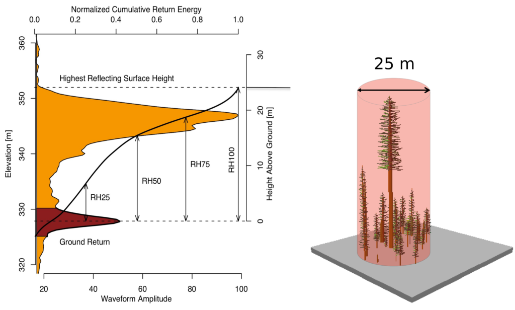
25 m

Data Latency

• Level 2A , 2B : 4 months in monthly intervals
• Level 4A , 4B : 6 months after global sampling required to meet L1 requirement

GEDI Configuration

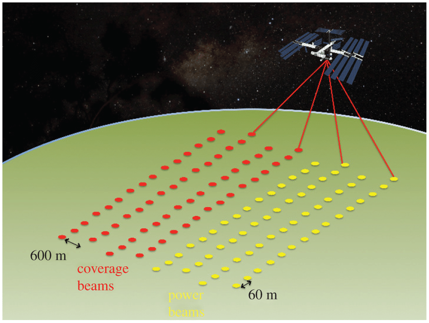
• The GEDI instrument consists of 3 lasers producing a total of 8 beam ground transects that are spaced approximately 600 m apart on the Earth’s surface in the cross-track direction relative to the flight direction, and approximately 735 m of zonal (parallel to lines of latitude) spacing.

• Thefundamental footprint observations made by the GEDI instrument are received waveforms of energy (number of photons) as a function of receive time.

• The GEDI waveforms are a distance measure of the vertical intercepted surfaces within a footprint. Captured within the receive outprint waveforms are the range to the ground and to various metrics of vegetation or “tree” height.

• The “coverage” laser is split into two transects that are then each dithered producing four ground transects. The other two lasers are dithered only, producing two ground transects each.

GEDI Waveform Overview

• A digitally-recorded return laser pulse, or waveform (Figure 2), represents the time history of the laser pulse as it interacts with the reflecting surfaces.

• The waveform can have a simple (single-mode) shape similar to that of the outgoing pulse [Fig. 2(a)] or be complex and multimodal with each mode representing a reflection from an apparently-distinct surface within the laser footprint (Figure 2(b)).

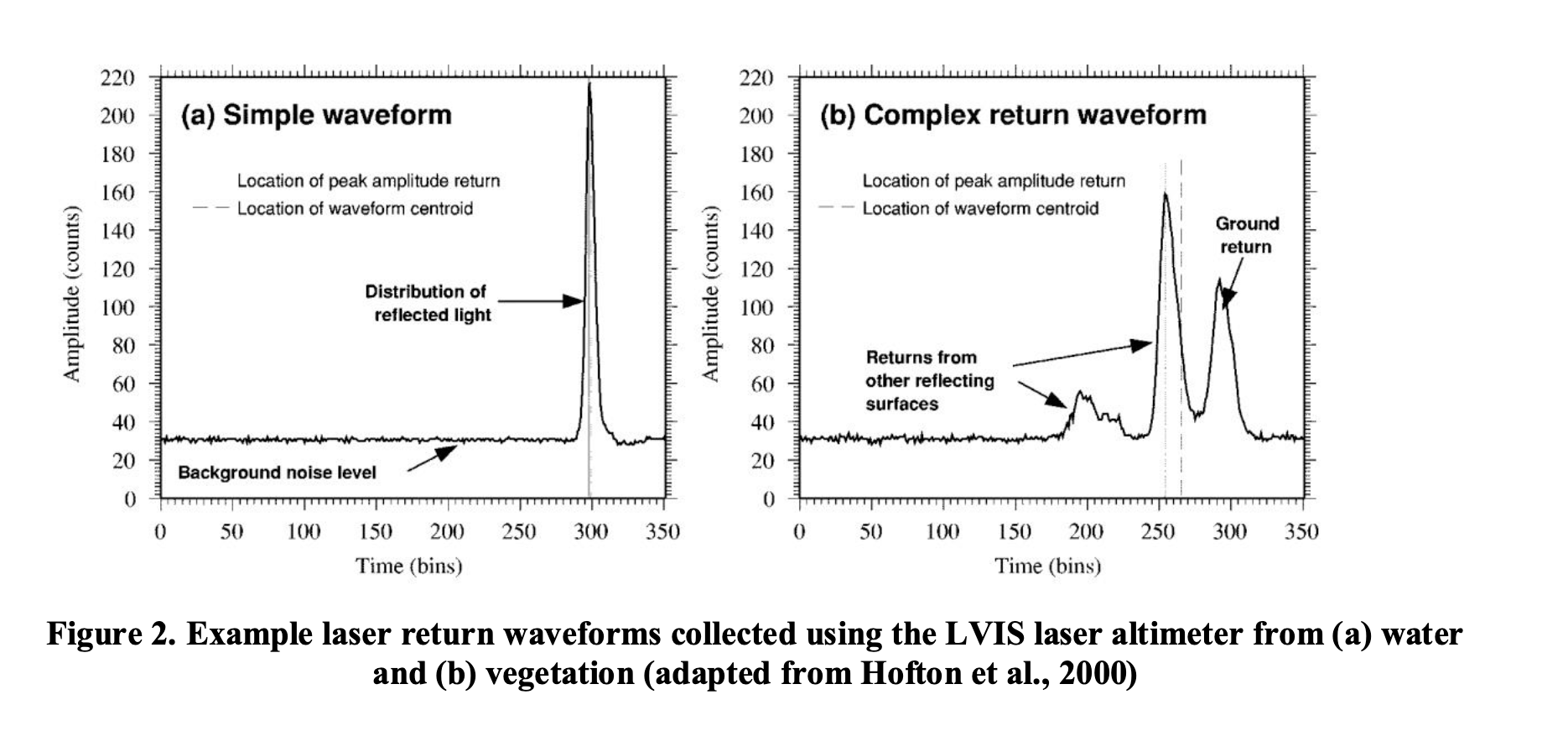
• Simple waveforms are typical in ocean or bare-ground regions.

• Complex waveforms in rough terrain or vegetated regions.

• The first and last modes (i.e., detected signal above noise) within the waveform are associated with the highest and lowest perceived reflecting surfaces within the footprint respectively.

Correcting Telemetered Transmit and Receive Waveforms for Known Artifacts

• The raw waveforms contain sampling artifacts (quantization, odd-even sampler offsets and both electronic and optical background noise.
• To minimize the impact of these we low pass filter the digital waveforms by convolution with a gaussian pulse. This reduces high frequency noise and effectively eliminates ADC sampling errors.
• The width of the gaussian pulse used for the convolution determines the amount of noise that is removed, but also loss of signal bandwidth (and the ability to detect multiple distinct pulses in the same waveform).

GEDI Receive Waveform Analysis

• “rx_assess” sub group of the L2A data product is the receive waveform, contain many infomation that we can interpret.
• But we need to characterize of the received pulse first (e.g., minimum and maximum amplitudes, energy).

1. Precise noise mean and noise standard deviation for each rxwaveform

Parameters: mean and sd_corrected

No additional refinement of noise statistics is currently performed, these are set to the values measured in real time by the sensor and are contained in the L1B data product.

2. Maximum and minimum amplitudes of the waveform

Parameters: rx_minamp and rx_maxamp

Measure the peak maximum and minimum amplitudes of the rxwaveform relative to the mean noise level.

3. Location of maximum amplitude return within waveform

Parameter: rx_maxpeakloc

Sample number of the maximum amplitude return (relative to bin0 of the rxwaveform).

4. Waveform amplitude clipping

Parameters: rx_clipbin_count, rx_clipbinnumber, and rx_clipbin0

When the signal levels exceed a certain intensity, the detector can no longer accurately represent the return signal and begins to act non-linearly (e.g., Sun et al., 2017), referred to as “saturation”. Because the detector does not accurately represent the return photon flux, information is distorted or lost. If this occurs in the vicinity or on the ground return then it will degrade the precision of the ground elevation and canopy height measurements. If it occurs anywhere in the waveform, other canopy metrics will be affected. We flag if the recorded waveform contains saturated intensities, the number of consecutive bins affected and the location of the first saturated bin. Externally-set thresholds are used to define saturation amplitudes, and are stored in ancillary/rx_clipamp. Saturated returns are rare.

5. Waveform total energy

Parameter: rx_energy

Rx pulse energy is estimated by computing the integrated area of the signal relative to the mean noise level. It’s computed by summing up the waveform amplitudes after subtracting the mean noise value.

6. Mean signal value within the 10k range window

Parameter: mean-64kadjusted

Average amplitude within 10km search window with energy from rxwaveform removed:

*mean_64kadjusted=(all_samples_sum-total(rxwaveform)) / (64.1024.-(rx_sample_count))

7. Laser shot used in measurement model calculations

Parameter: ocean_calibration_shot_flag

We provide a flag to indicate if the return waveform was used in the measurement model calculations over the ocean (see L1B ATBD).

8. Waveform Fidelity Flag

Parameter: rx_assess_flag

This is a bitfield of different flags with each bit indicating whether a condition is present/affected the real-time collection of the waveform.

9. Waveform Quality flag

Parameter: quality_flag

ndicates the waveform can be considered usable for downsteam analysis {1:yes; 0: no). This combines together a set of conditions to indicate the overall validity of a waveform for measuring surface structure. Pseudocode representing conditions that are combined to represent “good” conditions is:

• stale_return_flag == 0
• rx_rangewindow_clip_front == 0
• rx_rangewindow_clip_back == 0
• rx_clipflag == 0
• rx_rxwindow_limit == 0
• rx_rxwindow_exist != 0
• rx_rxwindow_clip_front == 0
• rx_rxwindow_clip_back == 0
• rx_1binwaveform_flag == 0
• rx_pulseflag != 0

Receive Waveform Interpretation

The purpose of the waveform interpretation algorithm is to derive timing points to which subsequent data products are referenced. The steps involved in interpretation of the RX pulse are:

• smooth the L1B “corrected” waveform
• using appropriate algorithm threshold settings, front and back, run interpretation algorithms
• in concert with L2A-geolocation, down select algorithm results.

The interpretation algorithm is adapted from that used on LVIS data since early 2000’s (Blair etal., 1999; LVIS, 2019)

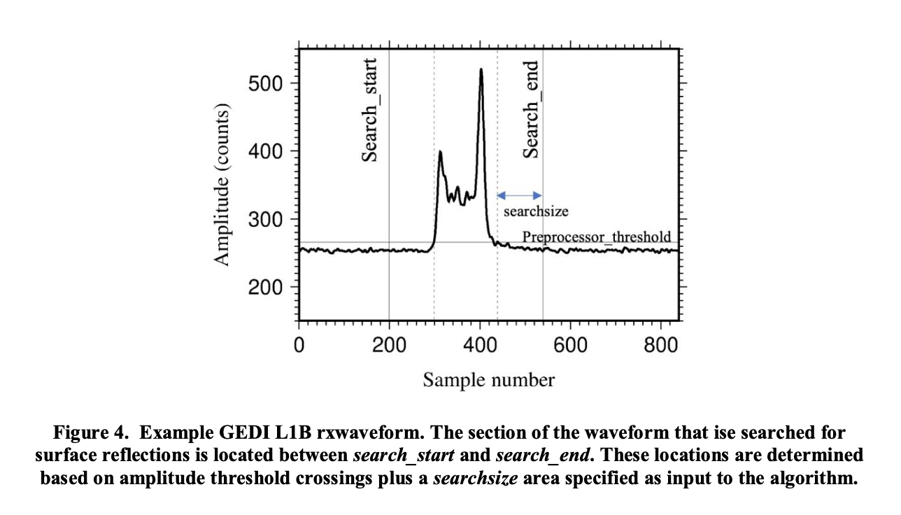
Determine signal extent within waveform

Parameters: search_start, search_end

We define the portion of the waveform to be searched for reflected signal based on the section of the waveform where intensity exceeds a threshold given by:

mean+sd_corrected x ancillary/preprocessor_threshold

This region is then extended immediately above and below by the number of samples set in ancillary/searchsize, modified to not exceed waveform record length as necessary. Search_start and search_end record the waveform sample numbers between which the algorithm will search for reflected signal (Figure 4),

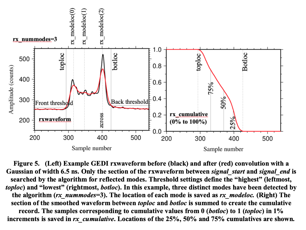
Parameters: Botloc, botloc_amp

Botloc (Figure 5) is defined as the lowest location in the section of the waveform between search_start and search_end where two adjacent intensities occur above back_threshold (Figure 5). This defines the lowest detectable return. Parameters are determined using the version of rxwaveform denoised by convolution with a gaussian of width smoothwidth. Botloc_amp is the intensity of the denoised waveform at the location of botloc.

Parameter: Toploc

Toploc (Figure 5) is defined as the highest detectable return where two adjacent intensities occur above front_threshold (Figure 5) within the section of the rxwaveform between search_start and search_end. Toploc defines the highest detected return. For example, in a vegetated area, this will correspond (once geolocated) to the canopy top. Parameters are determined from the version of rxwaveform denoised by convolution with a gaussian of width smoothwidth.

Detect modes within waveform

Parameters: rx_nummodes, rx_modeamps, rx_modelocs, rx_modewidths

The rxwaveform may contain several distinct modes representing reflecting surfaces within each laser footprint. An area of the rxwaveform denoised with a gaussian of width smoothwidth_zcross between search_start and search_end is searched (Figure 5). A mode is defined as a zero crossing

point of the first derivative of the de-noised waveform. Waveform intensity of the mode mus exceed back_threshold. A maximum of ancillary/max_mode_counts are stored. If the number of detected modes exceeds this value, no output from the algorithm is produced. Some of the detected modes may correspond to noise.

• Rx_nummodes: number of distinct modes detected by the algorithm
• Rx_modelocs: location of each distinct mode detected by the algorithm
• Rx_modeamps: intensity of de-noised waveform at corresponding rx_modelocs location.
• Rx_modewidths: estimate of width of each mode detected by algorithm, defined as the distance to the subsequent mode/2.

Waveform Sensitivity

Parameters: Min_detection_energy, min_detection_threshold

Due to atmospheric conditions that will vary from completely clear to completely clouded and all things in between, GEDI return signals will greatly vary in strength and, the ability to penetrate canopies is dependent on return signal strength. To aid in identifying waveforms where we may not have detected the true ground level (due to weak return signals and/or high density canopy cover), we compute a signal detection performance metric for the ground detection capability for each waveform, dubbed the “sensitivity” metric. Sensitivity is computed by simulating the minimum detectable ground return pulse energy for the given detection algorithm. The area of that return will be divided by the area for the total return waveform to produce the sensitivity parameter. This provides an estimate for the relative minimum percentage of the return that needs to be present in the ground return for it to be detected.

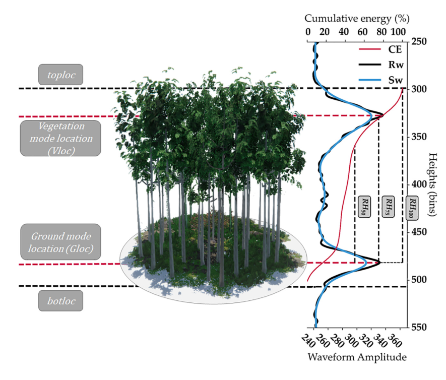
GEDI L2A Canopy Height

Simulated GEDI waveforms are processed to GEDI02_A equivalent relative height (RH) metrics, which are defined as the percentage of the received laser waveform intensity that is less than a given height, where height is computed relative to the elevation of the lowest mode in the waveform

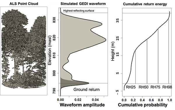
Figure : Relative height (RH) metrics were calculated as the height relative to ground elevation under which a certain percentage of waveform energy has been returned. RH50, for example, is the height relative to the ground elevation below which 50% of waveform energy has been returned.

GEDI L4A Footprint Level Aboveground Biomass

Global Ecosystem Dynamics Investigation (GEDI) Level 4A (L4A) contains predictions of the aboveground biomass density (AGBD; in Mg/ha) and estimates of the prediction standard error within each sampled geolocated laser footprint.

AGBD was derived from parametric models that relate simulated GEDI Level 2A (L2A) waveform relative height (RH) metrics to field plot estimates of AGBD.

Height metrics from simulated waveforms associated with field estimates of AGBD from multiple regions and plant functional types (PFTs) were compiled to generate a calibration dataset for models representing the combinations of world regions and PFTs (i.e., deciduous broadleaf trees, evergreen broadleaf trees, evergreen needleleaf trees, deciduous needleleaf trees, and the combination of grasslands, shrubs, and woodlands).

The GEDI approach to developing footprint AGBD models considers multiple candidates stratified by world region and PFT with different functional forms. The models were developed using a quality-filtered calibration dataset that contains 8,587 simulated waveforms in 21 countries. These data were contributed by numerous researchers and standardized into the GEDI FSBD, which is a living data archive that grows over time as new datasets are assimilated and improvements are made to existing records.

The GEDI04_A models are stratified by world region and PFT . Important regions are under-represented in the GEDI FSBD, including the forests of continental Asia, the evergreen broadleaf forests throughout the islands of Southeast Asia and north of Australia, and the worldwide distribution of savannas and deciduous tropical forests.

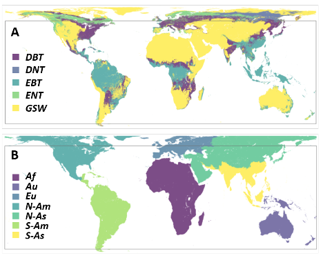
Figure : The GEDI04_A global stratification of plant functional types (PFT) (A) and world region (B) used to produce GEDI footprint AGBD models. The box inset is the GEDI observation domain of 51.6 degrees N to S latitude. PFT: DBT (deciduous broadleaf trees), DNT (deciduous needleleaf trees), EBT (evergreen broadleaf trees), ENT (evergreen needleleaf trees), GSW (grasses, shrubs, and woodlands). Regions: Af (Africa), Au (Australia and Oceania), Eu (Europe), N-Am (North America north of southern Mexico), N-As (North Asia), S-Am (South America, Central America, and southern Mexico, and the Caribbean), S-As (South Asia).

For each of the eight beams, additional data are reported with the AGBD estimates, including the associated uncertainty metrics, quality flags, model inputs, and other information about the GEDI L2A waveform for this selected algorithm setting group.

Model inputs include the scaled and transformed GEDI L2A RH metrics, footprint geolocation variables and land cover input data including PFTs and the world region identifiers. Additional model outputs include the AGBD predictions for each of the six GEDI L2A algorithm setting groups with AGBD in natural and transformed units and associated prediction uncertainty for each GEDI L2A algorithm setting group.

Example subset of aboveground biomass density (AGBD; Mg/ha-1) predictions from the GEDI Level-4A footprint product over Northern California, U.S., spanning April to July 2019. GEDI footprints are spaced 60m along-track and 600m across-track.

GEDI data format

GEDI raw data comes in the format of H5 one of the Hierarchical Data Formats (HDF) used to store large amount of data. It is used to store large amount of data in the form of multidimensional arrays. The format is primarily used to store scientific data that is well-organized for quick retrieval and analysis.

To retrive useful information. Only partials of layer need to be extracted.

Example of L2 product Layer

• /rh
• /elev_lowestmode
• /elev_highestreturn
• /lat_lowestmode
• /lon_lowestmode
• /shot_number
• /quality_flag
• /digital_elevation_model
• /degrade_flag
• /sensitivity
• /selected_algorithm

Tutorial and data access

GEDI data products are available at different site depends on level of product

• For Level 2, visit Land Processes Distributed Active Archive Center LPDAAC
• For Level 4, visit Oak Ridge National Laboratory Distributed Active Archive Center ORNLDAAC

For how-tos, and tutorials to help access and guideline to preprocess the data

• visit GEDI-L2A-Resources for level 2 product tutorials
• visit GEDI-L4A-Resources for level 4 product tutorials

Product are also available at Earth Engine Data Catalog

• L2A-EE
• L4A-EE